
What is Quantitative Easing?
Quantitative easing, or simply QE, is a central bank’s way to prop up an economy during a downturn. Central bankers do this by purchasing assets in the debt and equity capital markets in an attempt to lower interest rates. This sets off a domino effect in the economy. At first, QE feels good all around. But the hangover sets in the next morning.
A central bank’s buying bolsters the amount of money circulating in the economy, which, in turn, pressures interest rates lower, ultimately sparking lending activity to individuals and businesses. It is a way to artificially support the economy in the short term but eventually the time will come to pay the piper.
Quantitative easing was drummed up by German Economist Richard Werner in the mid-1990s. Japan’s quantitative easing program is widely considered the first formal use of this strategy. The Bank of Japan launched QE in March 2001 to combat deflation and a stagnant economy, years after the initial Asian Financial Crisis of 1997.
In the U.S., Ben Bernanke is the grandfather of QE. The former Federal Reserve Chairman implemented quantitative easing during the Great Financial Crisis of 2008.
Under Bernanke, the Fed created new bank reserves and used them to purchase bonds, commercial paper, and mortgage-backed securities. This expanded the money supply indirectly by flooding the banking system with liquidity, which banks could then lend out. Unlike direct money printing, QE works through financial markets and depends on banks and investors transmitting that liquidity into the broader economy.
It was under Bernanke’s expansive monetary policy that U.S. banking reserves ballooned from $870 billion prior to the GCF to $2.1 trillion. According to Bernanke, “The problem with QE is that it works in practice but it doesn’t work in theory.”
The Bank of England’s asset purchase facility (APF) balance sheet has similarly been expanding since 2009.
How QE Actually Works: A Step-by-Step Breakdown
QE sounds complex but the core mechanics follow a clear sequence. Here is how a typical QE program unfolds:
- Rates hit the floor: The central bank has already cut short-term interest rates to near zero and the economy still needs stimulus.
- Asset purchases begin: The central bank announces it will buy long-term government bonds (and sometimes mortgage-backed securities) from banks and financial institutions.
- Bank reserves expand: When the central bank buys a bond from a bank, it credits that bank’s reserve account with new funds. The bank now holds more reserves instead of a bond.
- Yields fall: Increased demand for bonds pushes prices up and yields down. This lowers borrowing costs across the economy, from mortgages to corporate loans.
- Portfolio rebalancing: Banks and investors who sold bonds now hold cash and seek higher returns in other assets like equities or real estate, pushing those prices up.
- Wealth and confidence effects: Rising asset prices increase household wealth and business confidence, encouraging spending and investment.
- Reinvestment phase: As purchased securities mature, the central bank reinvests proceeds to maintain the size of its balance sheet and sustain the stimulus effect.
Simple example: Before QE, a commercial bank holds $1 billion in government bonds. The central bank buys those bonds and credits the bank’s reserve account with $1 billion in new reserves. The bank’s assets shift from bonds to reserves. The central bank now holds the bonds on its balance sheet. The bank has more liquidity to lend, and bond yields across the market fall because the central bank’s buying has increased demand.
Quantitative Easing (QE) vs Quantitative Tightening (QT)
👉 Quick takeaway: QE expands the money supply to stimulate growth; QT shrinks it to fight inflation. Both have significant downstream effects on interest rates, asset prices, and borrowing costs.
| Feature | Quantitative Easing (QE) | Quantitative Tightening (QT) |
|---|---|---|
| Central Bank Action | Buys assets (bonds, MBS) | Sells assets or lets them mature without reinvesting |
| Effect on Money Supply |
🟢 Expands More reserves injected into system |
🔴 Contracts Reserves removed from system |
| Interest Rates | 🟢 Long-term rates fall | ⚠️ Long-term rates rise |
| Goal | Stimulate growth, fight deflation | Cool inflation, normalize policy |
| Effect on Stock Market |
🟢 Historically bullish Asset prices tend to rise |
⚠️ Historically creates headwinds for equities |
| Effect on Borrowing Costs | 🟢 Lower mortgage and loan rates | ⚠️ Higher mortgage and loan rates |
| Recent U.S. Example |
March 2020 Fed bought $120B/month in assets |
June 2022 Fed allowed up to $95B/month to roll off |
| Risk | ⚠️ Inflation, asset bubbles, wealth inequality | ⚠️ Recession risk, labor market pain, credit tightening |
When does the Fed switch from QE to QT?
The Fed typically follows this sequence:
- Taper QE purchases gradually (reduce monthly buying)
- Stop new purchases entirely
- Allow maturing securities to roll off the balance sheet without reinvestment
- Raise short-term policy rates alongside or after QT begins
According to Federal Reserve Bank of Atlanta research, a $2.2 trillion passive roll-off of nominal Treasury securities over three years is equivalent to approximately 29 basis points in rate hikes under normal conditions, and up to 74 basis points during turbulent periods.
Effects of Quantitative Easing
Quantitative easing is not all bad. There are some positive effects of this type of monetary easing. For example, macroeconomist and former Fed Governor Jeremy Stein once praised QE including large-scale asset purchases for playing a “significant role in supporting economic activity.” However, it is important to note that research from central banks have a tendency to be biased.
Other research has shown that QE in the U.S. economy after the GFC resulted in persistently lower interest rates on a number of assets and less credit risk. This dynamic resulted in stronger economic expansion but also inflation. Money flowed into equities and bolstered their valuations, ultimately widening the divide between high-net-worth individuals and the working class.
QE is credited with helping prevent a deflationary spiral in the eurozone. The European Central Bank launched its large-scale Public Sector Purchase Programme (PSPP) in March 2015, purchasing eurozone government bonds and other assets to push inflation toward its 2% target and compress sovereign bond yield spreads across member states. The Bank of Japan’s historic QE is said to have strengthened stock prices but did little to ignite corporate investment.
However, what goes up must come down. There are serious risks associated with QE, not least of which is high inflation. When the central bank turns the money printer to the “on” position, it inflates the dollar (or other fiat money) supply in the economy.
As a result, demand increases while the buying power of the dollar in circulation weakens, sending prices skyrocketing. QE could also have the intended consequence of acting as a steroid in the stock market, creating bubble-like conditions in equity valuations as well as in the real estate market. Investors lose their fear of risk and expect that the central bank will rescue them. According to investment bank UBS, in the 10 years leading up to 2019, returns on assets were highly correlated with the Fed’s QE programs.
Quantitative Easing Examples: U.S., Japan, and the Eurozone
- Quantitative easing was popular during the COVID-19 pandemic among central banks globally. Central banks across the U.S, Japan, the U.K., and the eurozone purchased approximately $10.2 trillion in securities assets, resulting in total assets on their balance sheets expanding to more than $25.9 trillion. According to the United Nations, these QE programs delivered “market liquidity” and an easing of “financial conditions in times of severe financial distress and market dysfunction.” In the U.S., the Fed began tapering its COVID-era asset purchases in late 2021 and launched formal quantitative tightening in June 2022 to combat the inflation that followed the pandemic-era stimulus. This QT phase involved allowing up to $95 billion per month in securities to roll off the balance sheet.
- On the heels of the Great Financial Crisis, the U.S. Fed implemented a QE program that lasted from 2009-2014. During this time, the Fed purchased assets like bonds and mortgages, resulting in its bank reserves surpassing $4 trillion by 2017.
- After Japan’s financial crisis in the late 1990s, the Bank of Japan formally launched quantitative easing in March 2001, making it the world’s first central bank to use this tool. The BoJ purchased government bonds, equities, and private debt in an effort to fight deflation and stimulate growth. The results were mixed. While the BoJ’s QE helped stabilize financial markets, Japan’s nominal GDP declined from approximately $5.45 trillion to $4.52 trillion during this period, partly due to persistent deflationary pressures and weak domestic demand that monetary policy alone could not overcome.
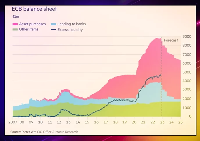
Below is an illustration of the ECB’s balance sheet and a forecast of the results of its quantitative tightening, as provided on Twitter by Philipp Heimberger, economist at the Vienna Institute for International Economic Studies. The original source of the image was Pictet WM CIO Office & Macro Research.
U.S. Federal Reserve QE Timeline
- QE1 (November 2008): Fed announced purchases of up to $600 billion in agency mortgage-backed securities and agency debt following the collapse of Lehman Brothers.
- QE2 (November 2010): Fed announced $600 billion in additional Treasury purchases at a pace of $75 billion per month.
- QE3 (September 2012): Open-ended program purchasing $40 billion per month in agency MBS, later expanded to $85 billion per month.
- COVID QE (March 2020): Fed announced unlimited asset purchases, initially buying $75 billion in Treasuries and $50 billion in MBS per day before settling at $120 billion per month.
- Taper (November 2021): Fed began reducing monthly purchases by $15 billion per month.
- QT (June 2022): Fed began allowing up to $47.5 billion per month (rising to $95 billion) to roll off its balance sheet.
FAQ: Common Questions About Quantitative Easing
Is QE the same as printing money?
Not exactly. When the Fed implements QE, it creates new bank reserves electronically and uses them to purchase assets like government bonds. This expands the central bank’s balance sheet and increases liquidity in the banking system. However, it is not the same as printing physical currency or directly funding government spending. The newly created reserves sit in the banking system and only enter the broader economy if banks lend them out.
Can QE cause high inflation?
It can, but the relationship is not automatic. QE expands bank reserves and lowers long-term interest rates, which can stimulate borrowing and spending. If that increased demand runs into limited supply, prices rise. However, during the post-2008 QE programs, inflation remained subdued for years because the economy was still weak and banks were not aggressively lending. The COVID-era QE contributed to inflation partly because it coincided with massive fiscal stimulus and supply chain disruptions, not QE alone.
How does the central bank exit QE?
The typical exit sequence is: (1) taper monthly asset purchases gradually, (2) stop new purchases entirely, (3) allow maturing securities to roll off the balance sheet without reinvestment (passive QT), and (4) raise short-term policy rates. The pace depends on economic data and inflation trends.
Does QE help ordinary people or just investors?
QE primarily works through financial markets first. Lower borrowing costs can help homeowners refinance mortgages and businesses access cheaper credit. However, the most immediate beneficiaries are holders of financial assets like stocks and real estate, which is why QE is frequently criticized for widening wealth inequality between asset owners and those without significant savings.
What QE Means for Your Investments and Savings
Understanding QE is useful. Knowing how to position around it is more useful. Here is how QE and QT have historically affected different asset classes:
During QE periods:
- Stocks: Historically bullish. UBS research found that in the 10 years to 2019, asset returns were highly correlated with Fed QE programs. The S&P 500 rose approximately 400% between QE1 (2008) and the end of QE3 (2014).
- Bonds: Prices rise as yields fall. Existing bondholders benefit. New buyers lock in lower yields.
- Real estate: Lower mortgage rates stimulate demand. Home prices rose significantly during post-2008 and post-2020 QE periods.
- Cash and savings accounts: Purchasing power erodes as inflation risk rises and savings rates fall near zero.
- Commodities: Often rise as the dollar weakens and inflation expectations increase.
During QT periods:
- Stocks: Historically face headwinds as liquidity is withdrawn and borrowing costs rise.
- Bonds: Prices fall as yields rise. Existing bondholders face paper losses.
- Real estate: Higher mortgage rates reduce affordability and can cool price growth.
- Cash: Savings rates improve as policy rates rise alongside QT.
Decision framework: Are you in a QE or QT environment?
- Check the Fed’s current balance sheet direction: expanding (QE) or contracting (QT)?
- Look at the federal funds rate trend: falling toward zero signals QE conditions; rising signals QT.
- Adjust portfolio duration and risk exposure accordingly.
Gerelyn

Gerelyn is a financial journalist who has been covering Wall Street for more than 20 years. After reporting for some of the top trade publications on investment banking, infrastructure and retirement, she was drawn to decentralization and shifted her coverage to the blockchain and cryptocurrency space in mid-2017. Since then, she has contributed to several major Bitcoin, Blockchain, and DeFi news sites, and has also written a children’s book.